Single Cell RNAseq Analysis
Steps
- Quality control
- Normalization
- Feature selection
- Dimensionality reduction
- Integration
- Clustering
- Annotation
Steps
- Quality control
- Normalization
- Feature selection
- Dimensionality reduction
- Integration
- Clustering
- Annotation
- Not necessarily a linear process
Quality Control
- Filter empty droplets
- Filter droplets with multiple cells
- Remove low quality cells
- Cells with high mitochondrial gene counts
- Suggests cell death or damage
- Filter cells with low gene counts
- Filter genes expressed in few cells
Quality Control
- Filter empty droplets
- Filter droplets with multiple cells
- Remove low quality cells
- Cells with high mitochondrial gene counts
- Suggests cell death or damage
- Filter cells with low gene counts
- Filter genes expressed in few cells
Quality Control
- Filter empty droplets
- Filter droplets with multiple cells
- Remove low quality cells
- Cells with high mitochondrial gene counts
- Suggests cell death or damage
- Filter cells with low gene counts
- Filter genes expressed in few cells
Quality Control
- Filter empty droplets
- Filter droplets with multiple cells
- Remove low quality cells
- Cells with high mitochondrial gene counts
- Suggests cell death or damage
- Filter cells with low gene counts
- Filter genes expressed in few cells
Quality Control
- Can set hard filtering thresholds
- These end up being arbitrary as there is rarely a clear boundary
- Time intensive
- Doesn’t scale well with large datasets
- Median Absolute Deviation (MAD) based filtering
- Uses the distribution of QC metrics to set thresholds
- More robust to outliers
- Can be automated
- MAD = median(|x - median(x)|), where x is the QC metric
Quality Control
- Best to be as permissive as possible
- Don’t want to filter out real cells
- Can always filter more later
- Iterative and data driven approach is best
- But beware of The garden of forking paths
- Why multiple comparisons can be a problem, even when there is no “fishing expedition” or “p-hacking”
- Be careful with your conclusions
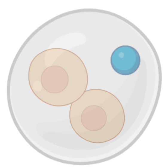
Doublet Detection
- Can be filtered out using tools like the
scDblFinder R package or Scrublet Python package
![]()
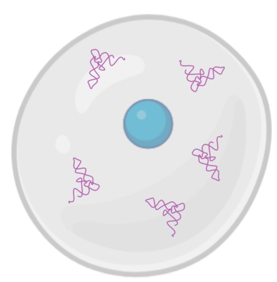
Correction of ambient RNA
- RNA in the environment of the cell
- Can be from dead cells, lysed cells, or other sources
- Potentially a significant source of noise in single cell RNAseq data
- Can be corrected for using tools like
SoupX
- These tools use the expression profiles of empty droplets to estimate the ambient RNA profile
- They then subtract this profile from the expression data of each cell
![]()
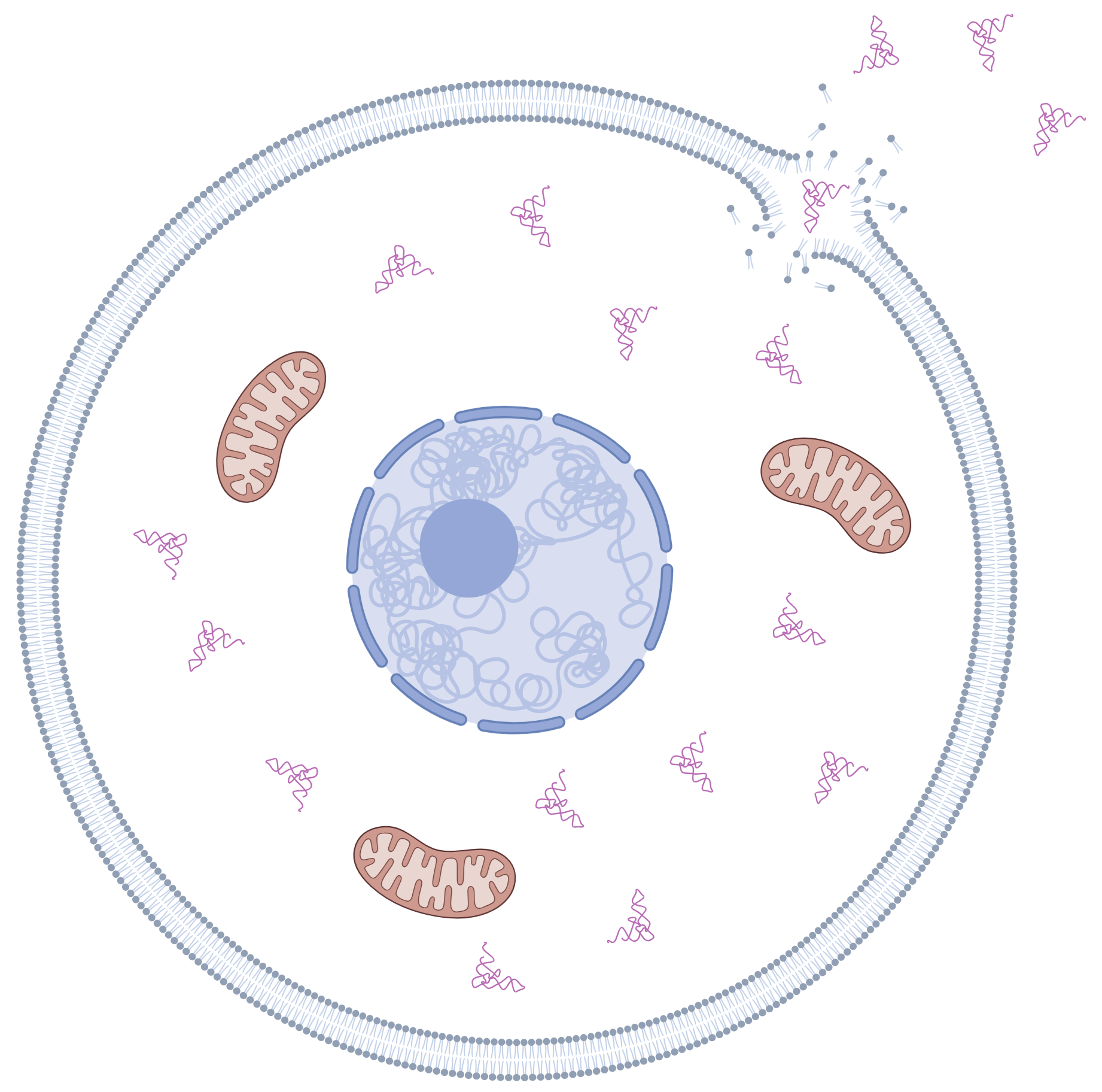
Normalization
- Each step of single cell workflow introduces a degree of variablity
- Capture of cells and mRNA molecules
- Reverse transcription
- Amplification
- Sequencing
- Count matrix contains widely varying variance terms
- Statistical methods assume uniform variance
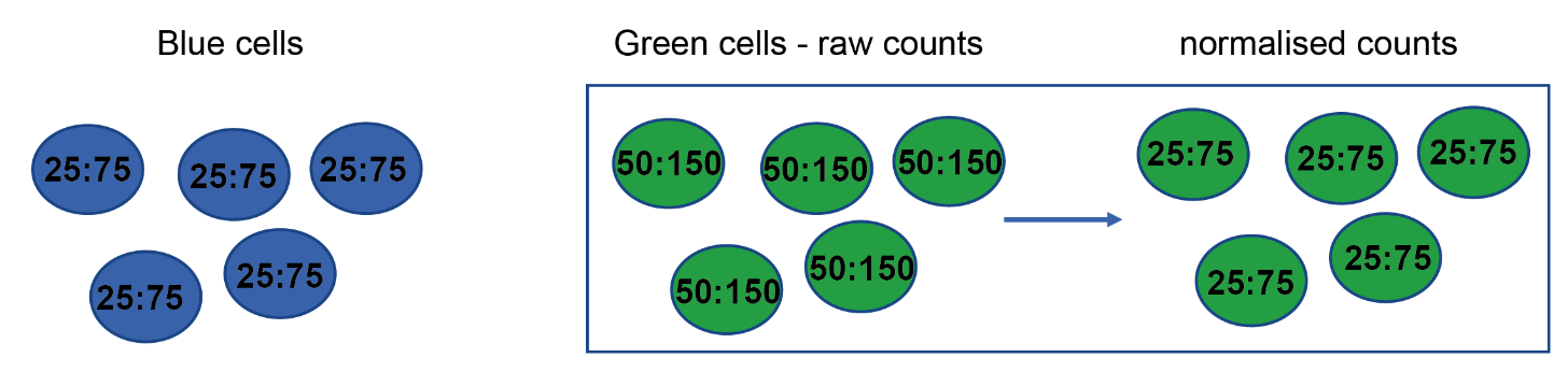
Normalization - Depth bias
- Two genes: A & B
- Two cell types: Blue & Green
- Normalize by dividing UMI counts for each gene by total
![]()
Cambridge Institute
- There is not differential expression, only a difference in sequencing depth
Normalization
- Normalization adjusts the raw counts by scaling to a specified range.
- Reduces technical differences so that differences between are primarily biological
- See Ahlmann-Eltze et al. 2020 for review & benchmarking of normalization methods
- Different techniques are better suited to different downstream analyses
Normalization - Techniques
- Shifted logarithm
- Works well for dimensionality reduction and differential expression
- Scran’s pooling-based size factor estimation method
- Works well or batch correction
- Analytic Pearson residuals
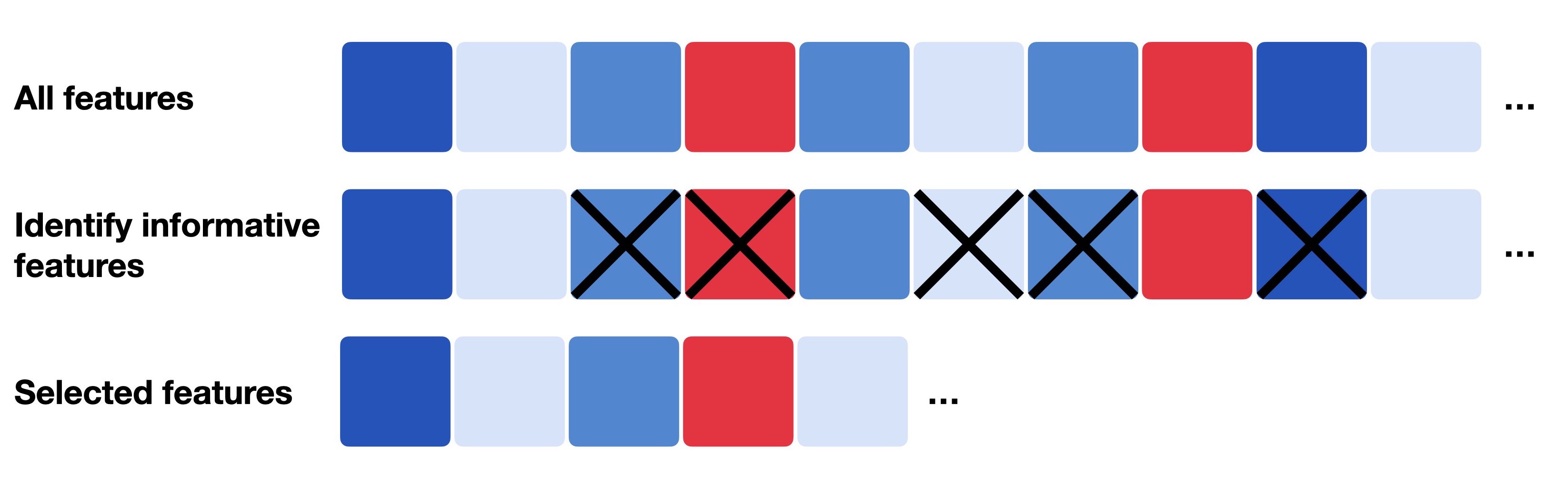
Feature Selection
- Many genes are not informative for downstream analysis
- We want to:
- Select gene that captue biologically meaningful variation
- Reduce the number of genes that only contribute noise
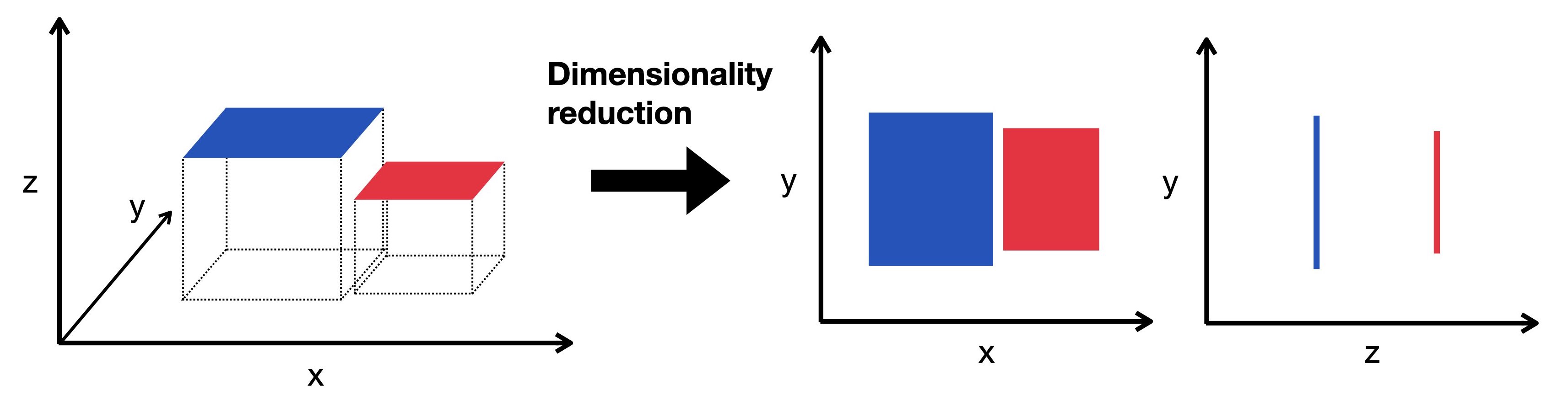
Dimensionality Reduction
- scRNAseq data suffers from the “curse of dimensionality”
- The data have a high number of dimensions (genes)
- Data contains more noise and redundancy
- Added dimensions do not add more information
Dimensionality Reduction
- We already reduced the dimensionality of the data by selecting a subset of genes
- We can reduce it further with dimensionality reduction algorithms
![]()
Luecken & Theis, 2019
- The most popular:
- Principal Component Analysis (PCA)
- t-distributed Stochastic Neighbor Embedding (t-SNE)
- Uniform Manifold Approximation and Projection (UMAP)
Principal Component Analysis (PCA)
- PCA creates new set of uncorrelated variables (principal components) that capture the most variance in the data
- The first principal component captures the most variance, the second captures the second most, and so on
- We can select the top principal components to use for downstream analysis
- Highly efficient and easy to interpret
- Not ideal for visualization
t-distributed Stochastic Neighbor Embedding (t-SNE)
- Graph based, non-linear dimensionality reduction technique
- Only local distances are preserved
- Stochastic, so results can vary between runs
- Good for visualizing clusters in high-dimensional data
- See StatQuest Video for a great explanation
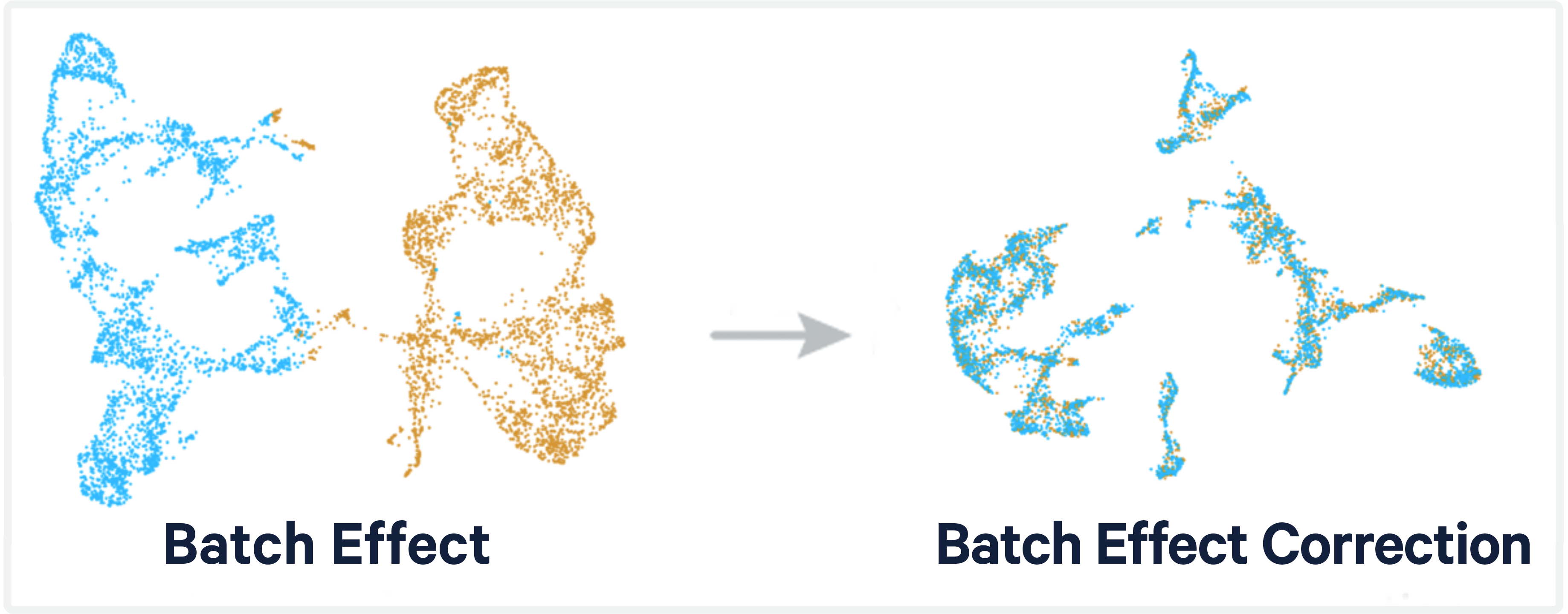
Integration
- Batch effects are a major challenge in scRNA-seq data analysis
- Arise from processing cells in separate batches
- Such as individual sample
- Obscure biological realities
- Removing batch effects is essential for analyses utlizing multiple batches
![]()
10X Genomics
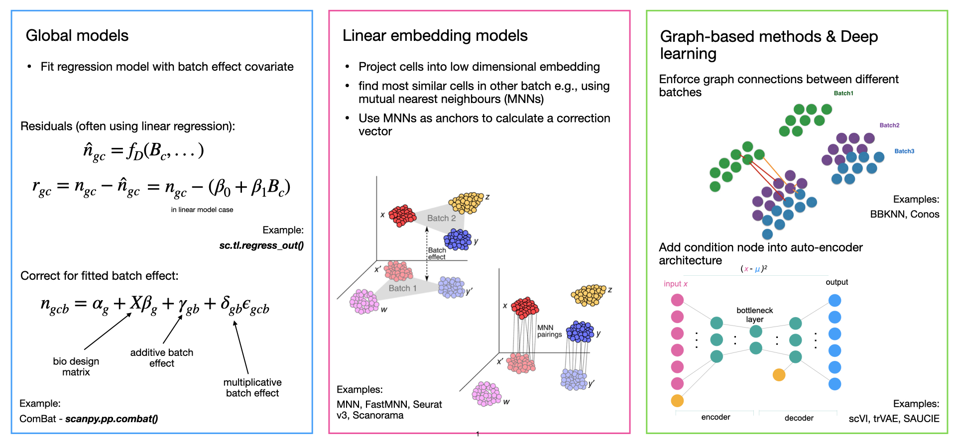
Integration
![]()
Luecken & Theis, 2019
Clustering
- Clustering is the process of grouping cells based on their expression profiles
- Common clustering algorithms:
- K-means
- Hierarchical clustering
- Louvain clustering
- Leiden clustering
- Louvain clustering was very popular for scRNA-seq data
- Leiden is now the preferred algorithm
- More robust to noise and outliers
- Better at detecting small clusters
- Clusters can be visualized with UMAP or t-SNE
Clustering
- Keep in mind:
- Clustering is an approximation of the underlying biological reality
- Different levels can be appropriate for different questions
- There may not be a single “correct” clustering
- Clustering algorithm will create as many cluster as you ask it to
- Don’t overlook continuous variation
Annotation
- Assigning cell types to clusters
- Can be done using:
- Marker genes
- Reference datasets
- Automated annotation tools
- Marker genes are genes that are specifically expressed in a particular cell type
- Reference datasets are datasets that have already been annotated
Steps
- Quality control
- Normalization
- Dimensionality reduction
- Clustering
- Integration
- Annotation